Colin Byrne

Single-Bit Response (SBR)

Methodology

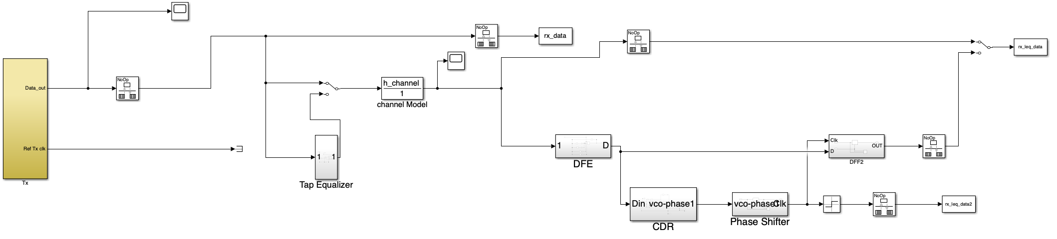
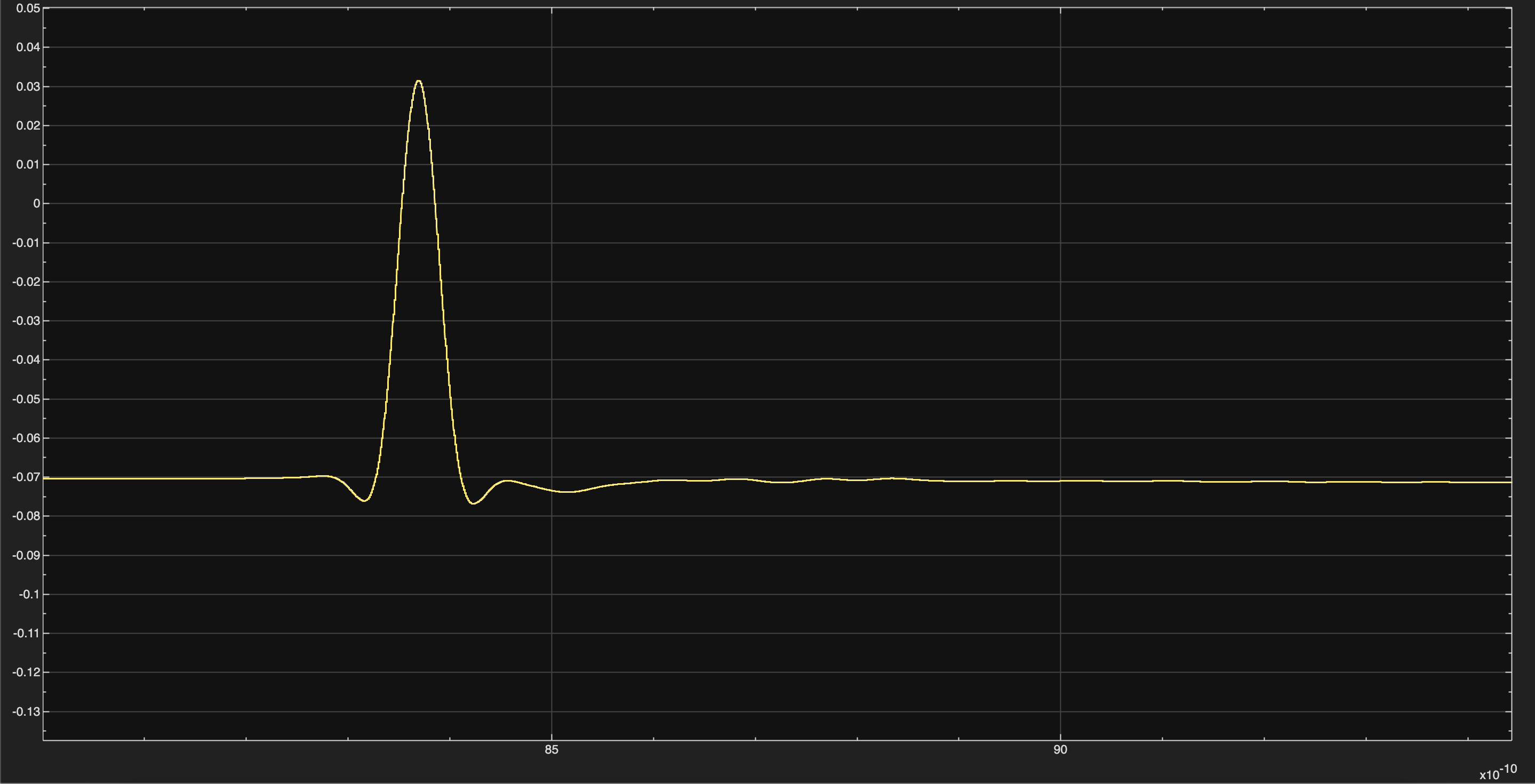
To generate the single-bit response (SBR), the channel impulse response provided in ELEC_4706_impulse.mat was loaded in MATLAB and used inside the discrete-time channel block of the Simulink model. A test sequence was created with all zeros and a single isolated 1 in the middle. This sequence was passed through the transmitter and channel path, and the resulting waveform after the channel was captured.

Pre- and post-cursor values were extracted using MATLAB scripts by sampling around the main cursor (maximum magnitude of normalized impulse response). The cursor set is denoted as [h_pre, h_0, h_post].

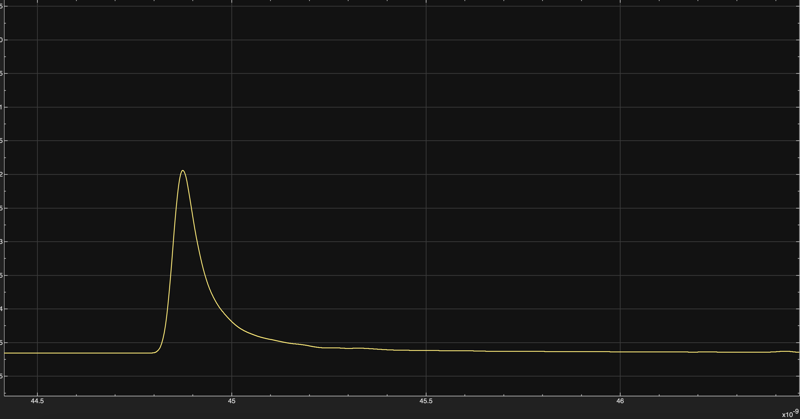
Generated Single-Bit Response

Pre- and Post-Cursors

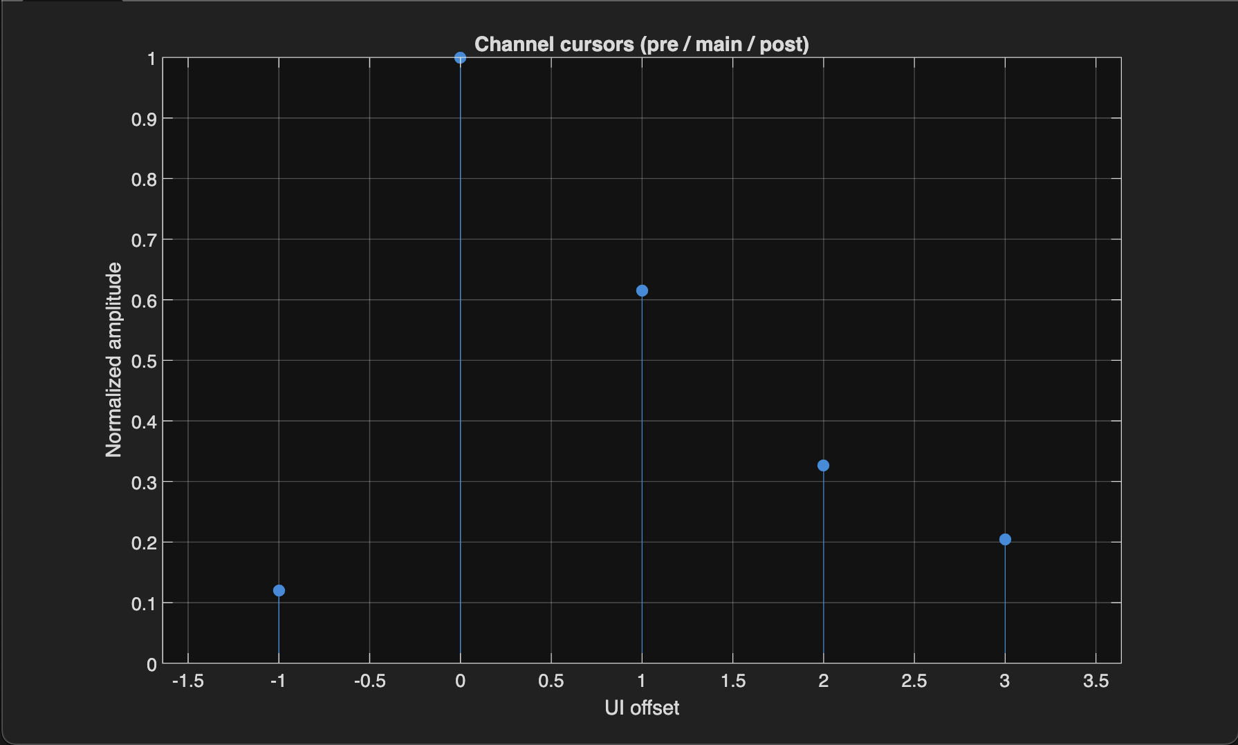
Calculated cursor values:

• \(h_0 = 0.5000\)
• \(h_1 = 0.0598\)
• \(h_{-1} = 0.3078\)
• \(h_{-2} = 0.1634\)
• \(h_{-3} = 0.1022\)

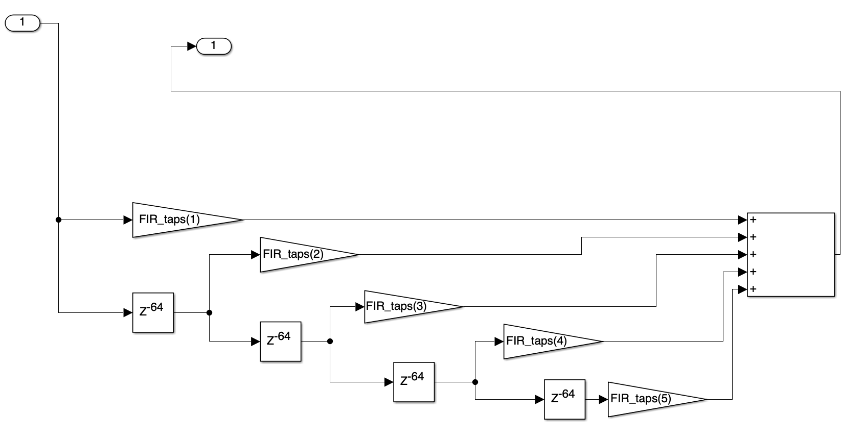
5-Tap Tx FIR and CTLE Equalization

Equalization Strategy

Continuous-time linear equalizer (CTLE) is applied at the receiver to boost high-frequency components. The transmitter uses a five-tap FIR filter to shape the waveform and minimize ISI. Tap coefficients are chosen to approximate \([0, 0, 1, 0, 0]\) after the channel.

Equalized Single-Bit Response

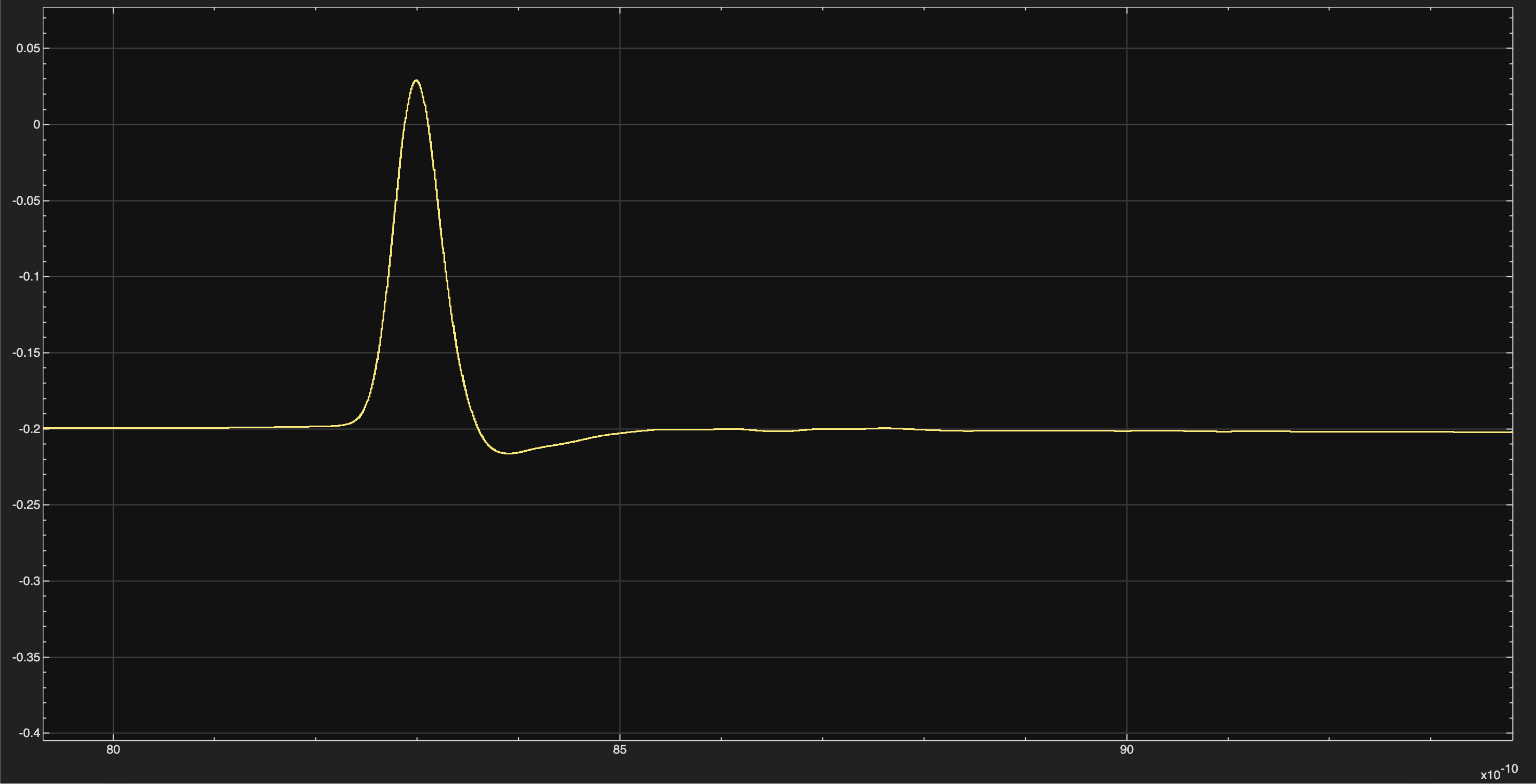
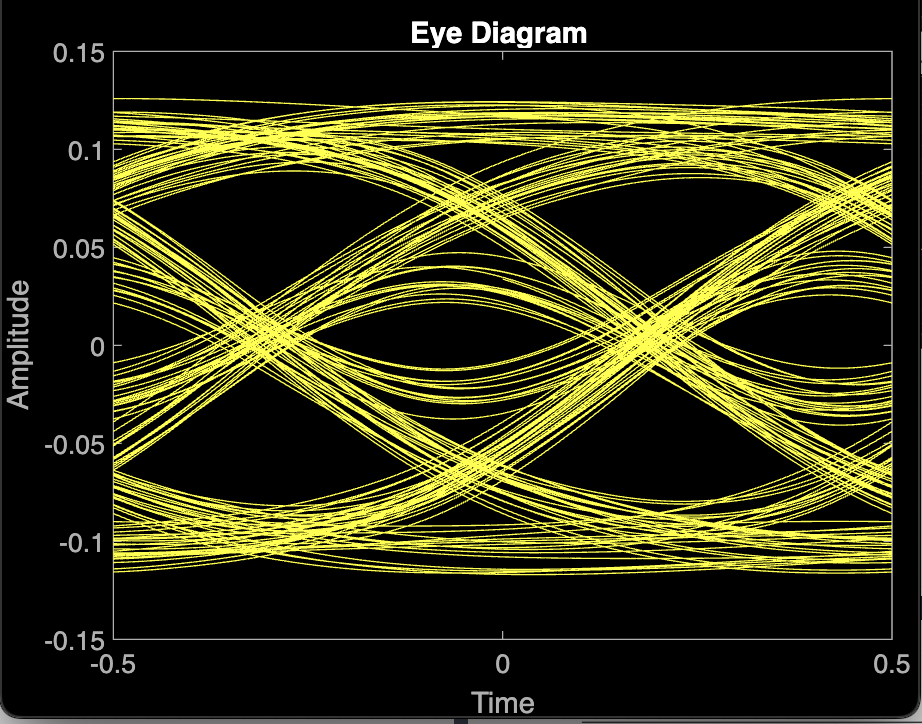
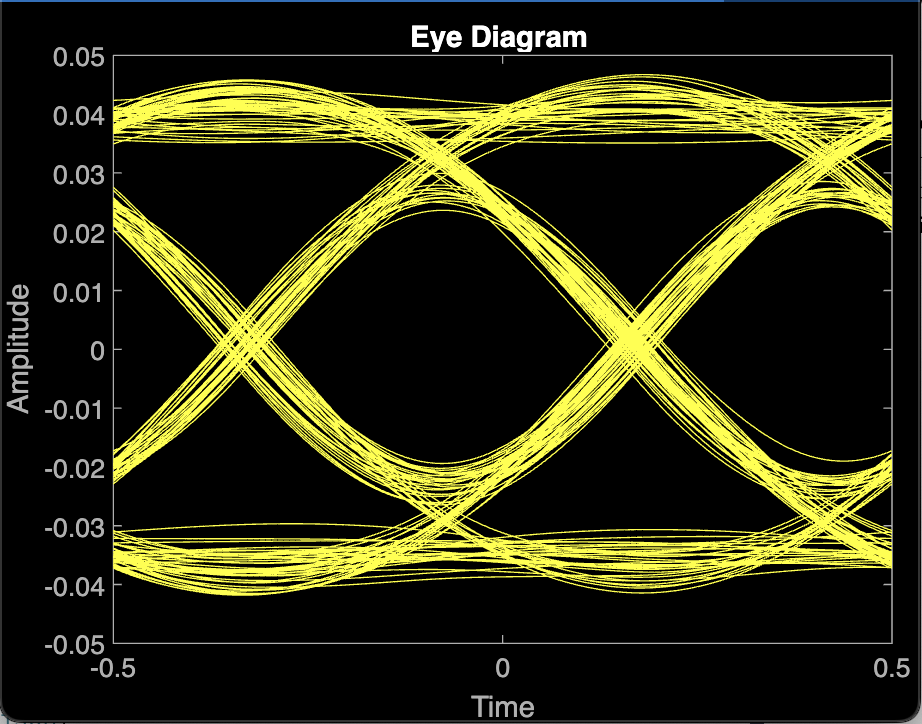
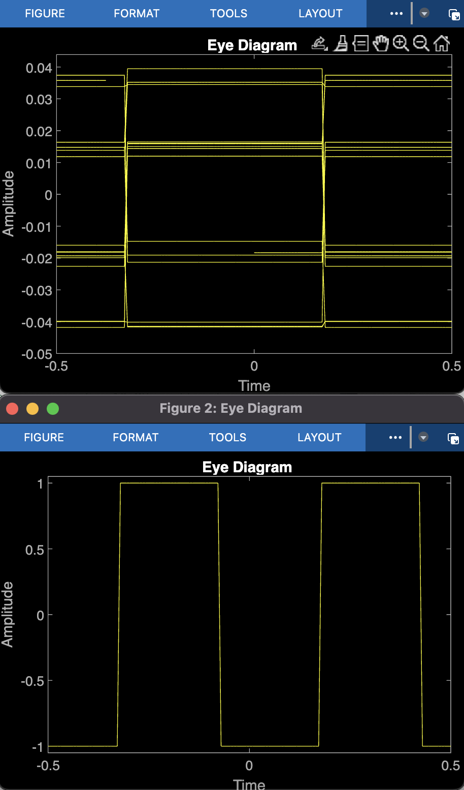
Eye Diagram Comparison

Justification

The combination of CTLE and five-tap FIR equalization produces a dominant main cursor and significantly reduces residual ISI, resulting in a cleaner and symmetric eye diagram suitable for 28 Gb/s operation.

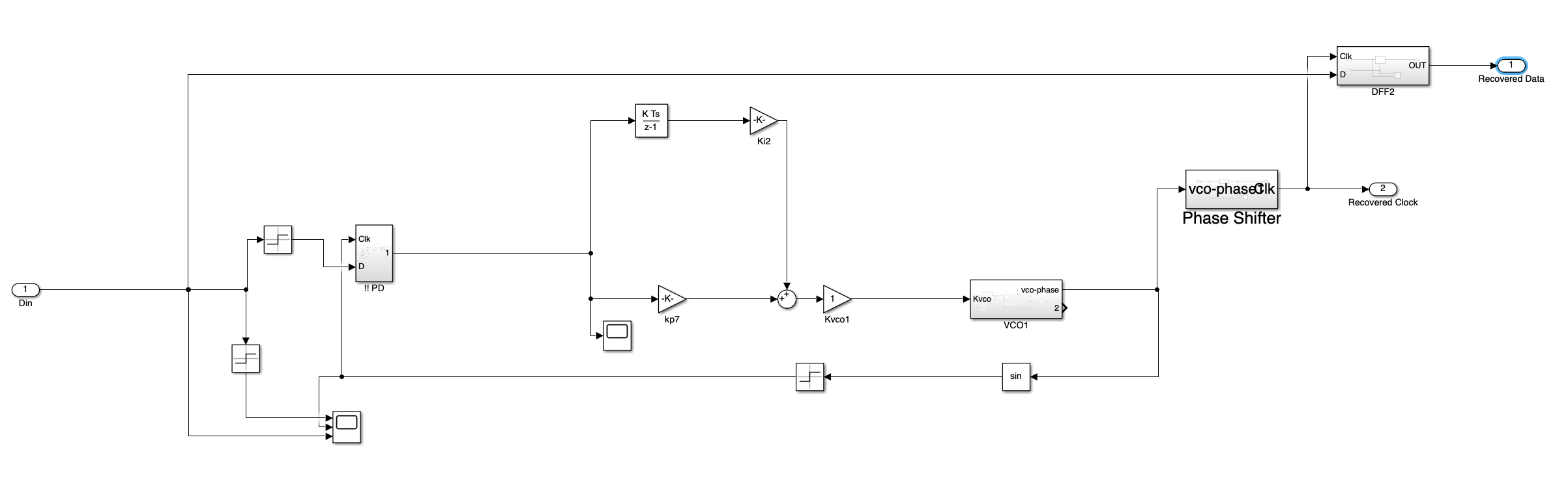
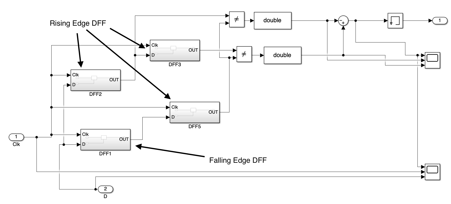
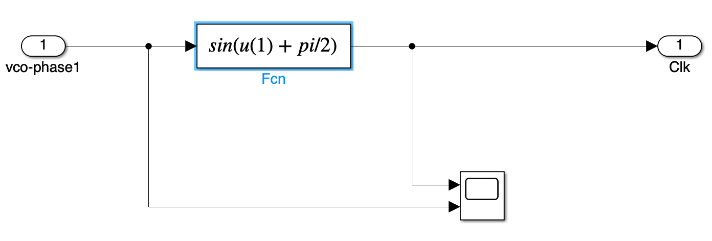
Timing Recovery and Phase Step Response

Timing Recovery / CDR Model

The digital bang-bang CDR loop recovers the clock from the data stream using Alexander phase detector, loop filter, VCO, and phase shifter. Gains were selected to achieve a 10 MHz jitter-tracking bandwidth.

Lock Point on the Eye Diagram

CTLE Design (4 dB High-Frequency Gain)

CTLE Transfer Function

The CTLE implements a one-zero, two-pole high-frequency boost:
\( H(s) = A_0 \frac{1 + s/\omega_z}{(1 + s/\omega_{p1})(1 + s/\omega_{p2})} \)

Pole and Zero Placement

Design targets a 4 dB gain at the Nyquist frequency (14 GHz). Selected values:

• \( f_z = 4.2 \text{ GHz} \)
• \( f_{p1} \approx 7.2 \text{ GHz} \)
• \( f_{p2} = 40 \text{ GHz} \)

Component Values

• \( R_z \approx 380 \Omega \)
• \( R_{p1} \approx 221 \Omega \)
• \( R_{p2} \approx 40 \Omega \)

Appendices

MATLAB Scripts

// MATLAB code used to generate the single-bit response
data_values1 = zeros(1, data_length1);

% Put a single '1' somewhere in the middle
one_index = 100; % choose a safe index, not at the very end
data_values1(one_index) = 1;

%% Find main, pre- and post-cursors from channel impulse
h = real(h_channel(:)).';

[~, idx_main] = max(abs(h));
h_norm = h / h(idx_main);

samples_per_UI = OSR;
N_pre  = 1;
N_post = 3;

ui_offsets   = -N_pre:N_post;
tap_indices  = idx_main + ui_offsets * samples_per_UI;
valid_mask   = tap_indices >= 1 & tap_indices <= length(h_norm);
ui_offsets   = ui_offsets(valid_mask);
tap_indices  = tap_indices(valid_mask);

taps = h_norm(tap_indices);

main_mask       = (ui_offsets == 0);
main_cursor     = taps(main_mask);

pre_mask        = (ui_offsets < 0);
pre_offsets_UI  = ui_offsets(pre_mask);
pre_cursors     = taps(pre_mask);

post_mask       = (ui_offsets > 0);
post_offsets_UI = ui_offsets(post_mask);
post_cursors    = taps(post_mask);

Tx_swing = 0.3;
h_0   = Tx_swing * main_cursor;
h_pre = Tx_swing * pre_cursors;
h_post = Tx_swing * post_cursors;

fprintf('\n=== Channel cursors (normalized, main = 1) ===\n');
fprintf('Main cursor (0 UI): % .4f\n', main_cursor);

Simulink Models